AI/ML

Diffusion Models

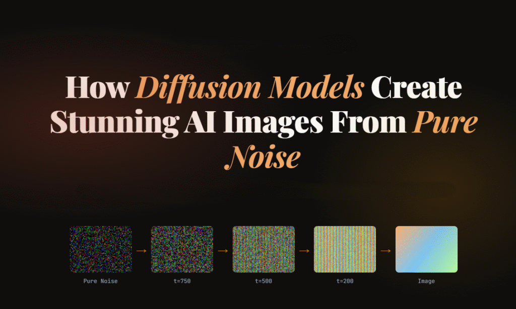
How Diffusion Models Create Stunning AI Images From Pure Noise

Artificial intelligence has changed digital creativity in ways that felt impossible just a few years ago. Today, AI can generate realistic portraits, cinematic landscapes, anime characters, product designs, and even paintings that look hand-crafted by professional artists.

At the center of this revolution are Diffusion Models.

These models power popular AI image generators like OpenAI DALL·E, Stability AI Stable Diffusion, and Google Imagen. What makes them fascinating is that they create detailed images starting from nothing but random noise.

Yes, literally noise.

In this guide, you’ll learn:

  • What Diffusion Models are
  • How they work step by step
  • Why they outperform older AI approaches
  • The mathematics behind the process
  • How text prompts become images
  • Real-world applications
  • Simple Python code examples
  • Challenges and future improvements

Everything is explained in a simple, beginner-friendly way with practical examples and easy-to-follow explanations.

What Are Diffusion Models?

Diffusion Models are a type of generative AI model designed to create new data, especially images, by gradually transforming random noise into meaningful visual content.

Think of it like sculpting.

An artist starts with a rough block of stone and slowly shapes it into a statue. Similarly, Diffusion Models begin with a chaotic noisy image and gradually refine it until a recognizable image appears.

The process happens in two stages:

  1. Forward Diffusion Process
    Noise is gradually added to training images until they become pure static.
  2. Reverse Diffusion Process
    The AI learns how to reverse the noise step-by-step to reconstruct realistic images.

That reverse process is where the magic happens.

Basically, for image generation, the model learns two things:

  1. How to slowly destroy an image by adding noise
  2. How to rebuild the image from that noise

During training, the model repeatedly sees images with different noise levels added to them. Over time, it learns how to predict and remove the noise accurately.

Once training is complete, the model can start from pure random static and generate entirely new images.

The name comes from physics: diffusion describes how particles spread from a concentrated point into a uniform distribution — like a drop of ink dispersing in water.

Diffusion models don’t “draw” an image directly. They learn to remove noise, one tiny step at a time, until a clean image emerges from what started as static.

Why Diffusion Models Became So Popular

Before Diffusion Models, GANs (Generative Adversarial Networks) dominated AI image generation. GANs produced impressive results but had several limitations:

  • Training instability
  • Mode collapse issues
  • Difficulty generating highly detailed scenes
  • Limited prompt understanding

Diffusion Models solved many of these problems.

Key Advantages of Diffusion Models

Better Image Quality

Diffusion-based systems generate sharper and more realistic images.

Stable Training

They are generally easier to train compared to GANs.

Strong Prompt Understanding

Modern Diffusion Models connect language and vision effectively.

Diverse Outputs

The same prompt can produce many unique results.

Scalable Architecture

They work well with massive datasets and larger neural networks.

Understanding the Core Idea With a Simple Analogy

Imagine placing a photograph into water and adding drops of ink repeatedly.

At first, the image is still visible.

Then it becomes blurry.

Eventually, it turns into complete chaos.

Now imagine training an AI to reverse that process perfectly.

The AI learns:

  • how much noise was added
  • where details originally existed
  • how edges, textures, and shapes should look

This is essentially how Diffusion Models work.

The Two Main Processes in Diffusion Models

1. Forward Diffusion Process

The forward process destroys the image slowly.

Mathematically, noise is added over many time steps.

The equation looks like this:

At every step:

  • a small amount of noise is added
  • the image becomes less recognizable
  • eventually only random static remains

After thousands of steps, the original image disappears completely.

2. Reverse Diffusion Process

This is where the AI generates images.

The model learns how to remove noise gradually.

Starting from random noise:

  • it predicts what the cleaner image should look like
  • removes a little noise
  • repeats the process many times

Eventually, a realistic image appears.

This reverse process is powered by deep neural networks trained on millions of images.

How Diffusion Models Learn During Training

Training teaches the model to predict noise accurately.

The process looks like this:

  1. Take a real image
  2. Add noise at different levels
  3. Ask the AI to predict the added noise
  4. Compare prediction with actual noise
  5. Improve the model through optimization

Over time, the AI becomes extremely good at reconstructing images from noisy inputs.

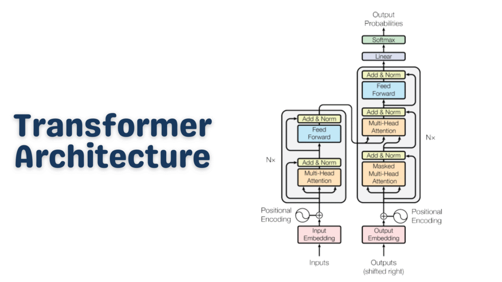
The Role of Neural Networks : U-Net

Most modern Diffusion Models use a neural network called a U-Net.

The U-Net architecture originally developed for medical image segmentation. The name comes from its shape: an encoder that compresses the input to a lower-resolution representation, followed by a decoder that brings it back to full resolution, with skip connections tying together the corresponding encoder and decoder layers at each scale.

The U-Net architecture helps the model:

  • understand image structures
  • preserve details
  • recover textures
  • maintain object consistency

It processes images at multiple resolutions simultaneously.

This allows the model to generate:

  • smooth faces
  • detailed hair
  • realistic lighting
  • accurate shadows
  • complex environments

How Text Prompts Become Images

One of the most impressive features of modern Diffusion Models is text-to-image generation.

For example:

“A futuristic cyberpunk city at night with neon rain.”

The AI converts that sentence into visual understanding.

Step-by-Step Prompt Processing

Step 1: Text Encoding

A language model converts the prompt into numerical vectors.

Step 2: Semantic Understanding

The AI learns relationships between words and visual patterns.

For example:

  • “cat” relates to fur, whiskers, ears
  • “sunset” relates to warm colors
  • “cyberpunk” relates to neon lighting and futuristic architecture

Step 3: Guided Image Generation

The diffusion process uses those text embeddings to guide image creation.

This is called conditioning.

What Is Latent Diffusion?

Modern systems like Stable Diffusion use Latent Diffusion Models (LDMs).

Instead of working directly on large images, the model compresses images into a smaller hidden representation called latent space.

Benefits include:

  • faster training
  • lower memory usage
  • improved efficiency
  • reduced computational cost

The process becomes:

  1. Compress image into latent space
  2. Perform diffusion there
  3. Decode back into full image

This innovation made AI image generation practical for consumer GPUs.

Simple Python Example of Diffusion Models

Let’s look at a simple Python example using the Hugging Face Diffusers library.

Install Required Libraries

Python
pip install diffusers transformers accelerate torch

Basic Text-to-Image Generation Code

Python
from diffusers import StableDiffusionPipeline
import torch

# Load model
pipe = StableDiffusionPipeline.from_pretrained(
    "runwayml/stable-diffusion-v1-5",
    torch_dtype=torch.float16
)

pipe = pipe.to("cuda")

# Text prompt
prompt = "A majestic dragon flying above snowy mountains"

# Generate image
image = pipe(prompt).images[0]

# Save image
image.save("dragon.png")
print("Image generated successfully!")

Explanation

Import Libraries

Python
from diffusers import StableDiffusionPipeline
import torch
  • diffusers provides pretrained Diffusion Models
  • torch handles deep learning operations

Load the Model

Python
pipe = StableDiffusionPipeline.from_pretrained(
    "runwayml/stable-diffusion-v1-5",
    torch_dtype=torch.float16
)

This downloads a pretrained Stable Diffusion model.

The model already understands:

  • objects
  • colors
  • lighting
  • styles
  • compositions

It has been trained on huge image-text datasets.

Move Model to GPU

Python
pipe = pipe.to("cuda")

This uses the GPU for faster image generation.

Without GPU acceleration, generation becomes much slower.

Define the Prompt

Python
prompt = "A majestic dragon flying above snowy mountains"

The text prompt guides the diffusion process.

More descriptive prompts usually produce better outputs.

Generate the Image

Python
image = pipe(prompt).images[0]

The model:

  1. starts with random noise
  2. removes noise gradually
  3. follows prompt guidance
  4. creates the final image

Save the Result

Python
image.save("dragon.png")

The generated image is stored locally.

What Happens Internally During Image Generation?

Behind the scenes, several advanced operations occur.

Noise Prediction

The model predicts which parts are noise.

Attention Mechanisms

Attention layers help connect text concepts to image regions.

For example:

  • “dragon” influences body structure
  • “snowy mountains” affects the background
  • “majestic” changes pose and atmosphere

Iterative Refinement

The image improves over many denoising steps.

Typical generation may use:

  • 20 steps
  • 50 steps
  • 100+ steps

More steps usually improve quality but increase generation time.

Sampling Methods in Diffusion Models

Different samplers control how noise removal happens.

Popular samplers include:

  • DDPM
  • DDIM
  • Euler
  • LMS
  • DPM++

Each sampler balances:

  • speed
  • realism
  • consistency

Some generate images faster, while others improve detail quality.

Classifier-Free Guidance Explained

Classifier-Free Guidance (CFG) controls prompt adherence.

Higher CFG values:

  • follow prompts more strictly
  • increase visual intensity
  • may reduce realism

Lower CFG values:

  • allow more creativity
  • produce softer interpretations

A common CFG range is:

7 to 12

Very high values can sometimes create oversaturated or distorted images.

Real-World Applications of Diffusion Models

Diffusion Models are transforming multiple industries.

Digital Art

Artists create concept art, illustrations, and fantasy scenes quickly.

Gaming

Studios generate textures, characters, and environments faster.

Marketing

Brands produce AI-generated advertisements and social media graphics.

Film Production

Filmmakers use AI for storyboarding and visual ideation.

Fashion Design

Designers experiment with clothing concepts instantly.

Medical Imaging

Researchers use diffusion techniques for image reconstruction and enhancement.

Architecture

Architects generate building concepts and interior visualizations.

Challenges and Limitations of Diffusion Models

Despite their power, Diffusion Models still face challenges.

High Computational Cost

Training requires enormous GPU resources.

Slow Generation Speed

Image creation involves many denoising iterations.

Bias in Training Data

Models may reproduce unwanted societal biases.

Copyright Concerns

Training datasets can contain copyrighted material.

Prompt Sensitivity

Small wording changes may produce very different outputs.

Ethical Considerations

AI-generated imagery raises important ethical questions.

These include:

  • misinformation
  • deepfakes
  • artist compensation
  • synthetic media transparency

Responsible AI development requires:

  • transparency
  • safety guardrails
  • dataset accountability
  • watermarking systems

Leading AI organizations continue researching safer generative systems.

Future of Diffusion Models

The future looks incredibly promising.

Researchers are improving:

  • generation speed
  • video generation
  • 3D object creation
  • real-time rendering
  • controllable outputs
  • multimodal AI systems

We are already seeing:

  • AI-generated movies
  • real-time editing tools
  • interactive creative assistants
  • AI-powered design workflows

Diffusion Models will likely become a core part of digital creativity across industries.

Frequently Asked Questions

Are Diffusion Models better than GANs?

In many cases, yes.

Diffusion Models generally produce:

  • more stable results
  • better detail quality
  • stronger prompt alignment

However, GANs can still be faster for some tasks.

Why do Diffusion Models start with noise?

Starting from noise allows the model to learn a flexible generative process capable of producing highly diverse outputs.

What is Stable Diffusion?

Stable Diffusion is an open-source latent diffusion model for generating images from text prompts.

Can Diffusion Models generate videos?

Yes.

Modern diffusion-based systems now support:

  • video generation
  • animation
  • frame interpolation
  • motion synthesis

Do Diffusion Models understand language?

Not directly like humans.

They learn statistical relationships between text and images using massive datasets.

Conclusion

Diffusion Models have fundamentally changed how machines create visual content.

What once required expert artists and expensive software can now be generated from a simple text prompt in seconds.

The idea is surprisingly elegant:

  1. destroy images with noise
  2. teach AI to reverse the destruction
  3. generate entirely new visuals from randomness

That simple concept powers some of the most advanced AI systems in the world today.

As computing power improves and research advances, Diffusion Models will continue reshaping art, design, entertainment, and digital creativity for years to come.

Transformer Architecture

Transformer Architecture Explained Simply: The AI Breakthrough Behind ChatGPT & Modern NLP

Have you ever wondered what actually powers ChatGPT, Google Translate, or GitHub Copilot under the hood? 

The answer is almost always the same: the Transformer architecture. It’s one of those rare inventions in computer science that didn’t just improve things a little — it completely rewrote the rules.

In this post, we’re going to break down the Transformer architecture from the ground up, without drowning you in intimidating math. Whether you’re a curious beginner or a developer looking to solidify your fundamentals, this guide is for you. Let’s dig in.

What Is the Transformer Architecture?

The Transformer architecture is a deep learning model design introduced in the landmark 2017 paper Attention Is All You Need by Vaswani et al. at Google. Before Transformers, most natural language processing (NLP) tasks relied on Recurrent Neural Networks (RNNs) and LSTMs (Long Short-Term Memory networks).

Those older models had a fundamental problem: they processed text word by word, in sequence. That means to understand the last word of a long sentence, the model had to “remember” everything that came before it — a bit like trying to recall the beginning of a movie after watching four hours of sequels.

The Transformer architecture threw that sequential approach out the window. Instead, it processes all words simultaneously and uses a clever mechanism called attention to understand relationships between words — no matter how far apart they are in a sentence.

That single change made everything faster, smarter, and more scalable.

Why Does Transformer Architecture Matter So Much?

Here’s a quick reality check: virtually every powerful AI language model you’ve heard of is built on the Transformer architecture.

  • ChatGPT → GPT-4 (Transformer-based)
  • Google Gemini → Transformer-based
  • Meta LLaMA → Transformer-based
  • BERT, T5, RoBERTa → All Transformer variants
  • GitHub Copilot → Powered by Codex (Transformer-based)

This isn’t a coincidence. The Transformer architecture solved problems that had been bottlenecking AI research for years — scalability, long-range dependencies, and parallelism. That’s why it became the standard almost overnight.

The Big Picture: How a Transformer Works

Before we go deep, let’s look at the 30,000-foot view.

Imagine you’re asking an AI: “What is the capital of France?”

Here’s what happens inside a Transformer:

  1. Your text gets broken into tokens (small pieces of text)
  2. Each token is converted into a vector (a list of numbers) — this is called an embedding
  3. The model adds positional information so it knows word order
  4. A series of encoder and/or decoder layers process these vectors
  5. Inside each layer, an attention mechanism figures out which words relate to which
  6. The output is a prediction — in this case, “Paris”

Simple, right? Now let’s zoom into each piece.

Tokenization: Breaking Text Into Pieces

Before the Transformer architecture can do anything, your text needs to be converted into tokens.

Tokens aren’t always full words. They can be sub-words, characters, or punctuation marks, depending on the tokenizer. For example:

Python
from transformers import GPT2Tokenizer

tokenizer = GPT2Tokenizer.from_pretrained("gpt2")
text = "Transformer architecture is amazing!"
tokens = tokenizer.encode(text)

print(tokens)
# Output: [8291, 16354, 10959, 318, 4998, 0]

decoded = tokenizer.decode(tokens)
print(decoded)
# Output: Transformer architecture is amazing!

Here,

  • We load a pre-trained GPT-2 tokenizer
  • We pass in a sentence and get back a list of integer IDs
  • Each integer maps to a specific token in the model’s vocabulary
  • The model never “reads” raw text — it only works with these numbers

This is the very first step in the Transformer pipeline. The richer and more consistent your tokenization, the better your model will perform.

Embeddings: Giving Numbers Meaning

Once we have token IDs, we convert them into embedding vectors — dense arrays of floating-point numbers that represent meaning.

Think of embeddings like coordinates on a map. Words with similar meanings cluster near each other in this high-dimensional space. “King” and “Queen” would be close together. “King” and “Broccoli” would be far apart.

Python
import torch
import torch.nn as nn

vocab_size = 50000   # Number of unique tokens
embed_dim  = 512     # Size of each embedding vector

embedding_layer = nn.Embedding(vocab_size, embed_dim)

# Simulate a batch of 2 sentences, each with 10 tokens
token_ids = torch.randint(0, vocab_size, (2, 10))
embeddings = embedding_layer(token_ids)

print(embeddings.shape)
# Output: torch.Size([2, 10, 512])
  • vocab_size is the total number of unique tokens the model knows
  • embed_dim = 512 means each token becomes a 512-dimensional vector
  • The output shape [2, 10, 512] means: 2 sentences × 10 tokens each × 512 numbers per token

These embeddings are learned during training — the model figures out the best numerical representation for each token by itself.

Positional Encoding: Telling the Model “Where” a Word Is

Here’s a subtle but critical issue: since the Transformer architecture processes all tokens at once (in parallel), it has no built-in sense of word order. “Dog bites man” and “Man bites dog” would look identical to it without some extra help.

That’s where positional encoding comes in. We add a special signal to each embedding that encodes its position in the sequence.

The original Transformer paper used sine and cosine functions for this:

Python
import torch
import math

def positional_encoding(seq_len, embed_dim):
    pe = torch.zeros(seq_len, embed_dim)
    position = torch.arange(0, seq_len).unsqueeze(1).float()
    
    # Division term creates different frequencies for each dimension
    div_term = torch.exp(
        torch.arange(0, embed_dim, 2).float() * 
        (-math.log(10000.0) / embed_dim)
    )
    
    # Even indices → sine, Odd indices → cosine
    pe[:, 0::2] = torch.sin(position * div_term)
    pe[:, 1::2] = torch.cos(position * div_term)
    
    return pe

pe = positional_encoding(seq_len=10, embed_dim=512)
print(pe.shape)
# Output: torch.Size([10, 512])

Why sine and cosine?

  • They produce unique patterns for every position
  • The model can generalize to sequences longer than what it saw during training
  • Nearby positions have similar encodings, which helps the model understand proximity

You simply add this positional encoding to your embeddings before passing them into the Transformer layers. The model then bakes position awareness into everything it computes.

The Heart of It All: The Attention Mechanism

This is where the magic lives. The self-attention mechanism is the defining feature of the Transformer architecture — and the reason it leaves RNNs in the dust.

Self-attention lets every token in a sequence “look at” every other token and decide: “How relevant is that word to understanding me?”

For example, in the sentence:

“The bank by the river flooded after the rain.”

When the model processes the word “bank”, attention lets it look at “river” and “flooded” to understand that “bank” here means a riverbank — not a financial institution. That’s context-awareness in action.

Query, Key, and Value — The QKV Framework

Attention is computed using three matrices: Query (Q), Key (K), and Value (V).

Here’s the intuition:

  • Query: “What am I looking for?”
  • Key: “What do I have to offer?”
  • Value: “What information do I actually carry?”
Python
import torch
import torch.nn.functional as F

def scaled_dot_product_attention(Q, K, V):
    """
    Q: Query matrix  → shape [batch, seq_len, d_k]
    K: Key matrix    → shape [batch, seq_len, d_k]
    V: Value matrix  → shape [batch, seq_len, d_v]
    """
    d_k = Q.size(-1)  # Dimension of the key vectors
    
    # Step 1: Compute raw attention scores (dot product of Q and K)
    scores = torch.matmul(Q, K.transpose(-2, -1))
    
    # Step 2: Scale to prevent huge values (which cause vanishing gradients)
    scores = scores / math.sqrt(d_k)
    
    # Step 3: Convert scores to probabilities with softmax
    attention_weights = F.softmax(scores, dim=-1)
    
    # Step 4: Multiply weights by values to get the output
    output = torch.matmul(attention_weights, V)
    
    return output, attention_weights

# Quick test
batch_size, seq_len, d_k = 2, 10, 64
Q = torch.rand(batch_size, seq_len, d_k)
K = torch.rand(batch_size, seq_len, d_k)
V = torch.rand(batch_size, seq_len, d_k)

output, weights = scaled_dot_product_attention(Q, K, V)

print(output.shape)    # torch.Size([2, 10, 64])
print(weights.shape)   # torch.Size([2, 10, 10])  ← attention map

This function implements scaled dot-product attention, a core idea behind Transformer models like GPT and BERT.

It works by comparing each query (Q) with all keys (K) using a dot product to measure similarity. These scores are then scaled (to keep values stable), passed through a softmax to turn them into probabilities, and used to weight the values (V).

The result is that each element in the sequence gathers relevant information from other elements, allowing the model to focus on what matters most.

The output of attention for each token is a weighted blend of all other tokens’ information, where the weights tell us how much to pay attention to each one.

Multi-Head Attention: Looking From Many Angles

One attention head is great, but different heads can learn to focus on different types of relationships simultaneously.

One head might focus on syntax. Another might focus on coreference (who “she” refers to). Another might track sentiment. This is Multi-Head Attention.

Python
import torch.nn as nn
import math

class MultiHeadAttention(nn.Module):
    def __init__(self, embed_dim, num_heads):
        super().__init__()
        assert embed_dim % num_heads == 0, "embed_dim must be divisible by num_heads"
        
        self.num_heads = num_heads
        self.head_dim  = embed_dim // num_heads  # Each head gets a slice of the embedding
        self.embed_dim = embed_dim
        
        # Single projection matrices for all heads combined (efficient!)
        self.W_q = nn.Linear(embed_dim, embed_dim)
        self.W_k = nn.Linear(embed_dim, embed_dim)
        self.W_v = nn.Linear(embed_dim, embed_dim)
        self.W_o = nn.Linear(embed_dim, embed_dim)  # Final output projection
    
    def split_heads(self, x):
        """Reshape from [batch, seq, embed_dim] → [batch, heads, seq, head_dim]"""
        batch, seq, _ = x.size()
        x = x.view(batch, seq, self.num_heads, self.head_dim)
        return x.transpose(1, 2)
    
    def forward(self, x):
        # Project input to Q, K, V
        Q = self.split_heads(self.W_q(x))
        K = self.split_heads(self.W_k(x))
        V = self.split_heads(self.W_v(x))
        
        # Scaled dot-product attention for all heads at once
        d_k    = Q.size(-1)
        scores = torch.matmul(Q, K.transpose(-2, -1)) / math.sqrt(d_k)
        weights = torch.softmax(scores, dim=-1)
        attn_output = torch.matmul(weights, V)
        
        # Merge heads back: [batch, heads, seq, head_dim] → [batch, seq, embed_dim]
        batch, _, seq, _ = attn_output.size()
        attn_output = attn_output.transpose(1, 2).contiguous()
        attn_output = attn_output.view(batch, seq, self.embed_dim)
        
        # Final linear projection
        return self.W_o(attn_output)

# Test it
mha = MultiHeadAttention(embed_dim=512, num_heads=8)
x   = torch.rand(2, 10, 512)   # [batch=2, seq_len=10, embed_dim=512]
out = mha(x)
print(out.shape)
# Output: torch.Size([2, 10, 512])

This implements multi-head attention, an extension of scaled dot-product attention.

Instead of performing attention once, the input is projected into multiple smaller “heads,” each learning different relationships in the data. Attention is computed in parallel across these heads, and the results are then combined and projected back to the original dimension.

This allows the model to capture diverse patterns (e.g., syntax, context, long-range dependencies) more effectively than a single attention operation.

What to notice:

  • num_heads=8 means we split the 512-dim embedding into 8 heads of 64 dims each
  • Each head runs attention independently on its own slice
  • The results are concatenated and passed through a final linear layer
  • The output shape is identical to the input — clean and composable

Feed-Forward Network: Processing Each Token Individually

After attention, each token’s representation passes through a small feed-forward network (FFN) — independently and identically for every position.

Think of this as a per-token “thinking step” where the model deepens its understanding after gathering context via attention.

Python
class FeedForward(nn.Module):
    def __init__(self, embed_dim, ff_dim, dropout=0.1):
        super().__init__()
        self.net = nn.Sequential(
            nn.Linear(embed_dim, ff_dim),   # Expand: 512 → 2048
            nn.ReLU(),                       # Non-linearity
            nn.Dropout(dropout),             # Regularization
            nn.Linear(ff_dim, embed_dim),   # Contract: 2048 → 512
        )
    
    def forward(self, x):
        return self.net(x)

ffn = FeedForward(embed_dim=512, ff_dim=2048)
x   = torch.rand(2, 10, 512)
print(ffn(x).shape)
# Output: torch.Size([2, 10, 512])

The FFN expands the dimensionality (typically 4×), applies a non-linearity, then contracts back. This expansion gives the model extra “room to think” before compressing its insight back into the embedding.

Layer Normalization & Residual Connections

You’ve probably noticed that deep neural networks can be tricky to train — gradients explode or vanish, and small errors compound. The Transformer architecture tackles this with two simple but powerful tricks: residual connections and layer normalization.

Python
class TransformerBlock(nn.Module):
    def __init__(self, embed_dim, num_heads, ff_dim, dropout=0.1):
        super().__init__()
        self.attention = MultiHeadAttention(embed_dim, num_heads)
        self.ffn       = FeedForward(embed_dim, ff_dim, dropout)
        self.norm1     = nn.LayerNorm(embed_dim)
        self.norm2     = nn.LayerNorm(embed_dim)
        self.dropout   = nn.Dropout(dropout)
    
    def forward(self, x):
        # Sub-layer 1: Multi-Head Attention + Residual + Norm
        attn_out = self.attention(x)
        x = self.norm1(x + self.dropout(attn_out))  # "Add & Norm"
        
        # Sub-layer 2: Feed-Forward + Residual + Norm
        ffn_out = self.ffn(x)
        x = self.norm2(x + self.dropout(ffn_out))   # "Add & Norm"
        
        return x

block = TransformerBlock(embed_dim=512, num_heads=8, ff_dim=2048)
x     = torch.rand(2, 10, 512)
out   = block(x)
print(out.shape)
# Output: torch.Size([2, 10, 512])

Why residual connections?

The x + sub_layer(x) pattern means the model adds the sub-layer’s output to its original input. If the sub-layer learns nothing useful, the input passes through unchanged — a built-in safety net that makes training much more stable.

Why layer normalization?

It normalizes the values inside each layer to have a mean of 0 and a standard deviation of 1. This keeps numbers in a healthy range throughout the network and speeds up training significantly.

Encoder vs. Decoder: Two Flavors of Transformer

The original Transformer architecture had both an encoder and a decoder, each serving a distinct role.

The Encoder

Reads the input and builds a rich contextual understanding of it. It uses bidirectional attention — every token can attend to every other token freely. Models like BERT are encoder-only.

Best for: Classification, named entity recognition, question answering (extractive)

The Decoder

Generates output one token at a time. It uses masked self-attention — when generating token #5, it can only look at tokens 1–4, not future ones. GPT models are decoder-only.

Best for: Text generation, autocomplete, creative writing, code generation

Encoder-Decoder (Seq2Seq)

Uses both halves together. The encoder processes the input; the decoder generates the output while attending to the encoder’s output. T5 and the original translation Transformers fall here.

Best for: Translation, summarization, question generation

Putting It All Together: A Minimal Transformer

Here’s a simplified but complete Transformer encoder that strings together everything we’ve covered:

Python
class SimpleTransformerEncoder(nn.Module):
    def __init__(
        self,
        vocab_size,
        embed_dim,
        num_heads,
        ff_dim,
        num_layers,
        max_seq_len,
        dropout=0.1
    ):
        super().__init__()
        self.embedding         = nn.Embedding(vocab_size, embed_dim)
        self.positional_encode = nn.Embedding(max_seq_len, embed_dim)  # Learned positional encoding
        self.layers            = nn.ModuleList([
            TransformerBlock(embed_dim, num_heads, ff_dim, dropout)
            for _ in range(num_layers)
        ])
        self.norm    = nn.LayerNorm(embed_dim)
        self.dropout = nn.Dropout(dropout)
    
    def forward(self, token_ids):
        batch, seq_len = token_ids.shape
        
        # Create position indices [0, 1, 2, ..., seq_len-1]
        positions = torch.arange(seq_len, device=token_ids.device).unsqueeze(0)
        
        # Combine token embeddings + positional embeddings
        x = self.dropout(
            self.embedding(token_ids) + self.positional_encode(positions)
        )
        
        # Pass through each Transformer block
        for layer in self.layers:
            x = layer(x)
        
        return self.norm(x)  # Final normalization

# Build a small model
model = SimpleTransformerEncoder(
    vocab_size   = 10000,
    embed_dim    = 256,
    num_heads    = 8,
    ff_dim       = 1024,
    num_layers   = 4,
    max_seq_len  = 128
)

# Simulate a batch of token IDs
token_ids = torch.randint(0, 10000, (2, 20))  # Batch of 2, length 20
output    = model(token_ids)
print(output.shape)
# Output: torch.Size([2, 20, 256])

# Count parameters
total_params = sum(p.numel() for p in model.parameters())
print(f"Total parameters: {total_params:,}")
# Output: Total parameters: ~7,000,000

What you’re seeing:

  • vocab_size=10000 → 10,000 unique tokens
  • embed_dim=256 → each token is a 256-dim vector
  • num_heads=8 → 8 parallel attention heads
  • num_layers=4 → 4 stacked Transformer blocks
  • The output is [2, 20, 256] — contextual representations for every token

Stack more layers, add more heads, and use bigger embeddings — that’s essentially how you scale from this toy model to something like GPT-4.

Common Transformer Variants You Should Know

The Transformer architecture has spawned an entire family of specialized models. 

The core Transformer architecture is the same backbone in all of them — the differences are in training objectives, scale, and fine-tuning strategies.

Key Strengths of the Transformer Architecture

Let’s summarize why this architecture won:

Parallelism — Processes all tokens simultaneously, making it GPU-friendly and fast to train.

Long-range dependencies — Attention connects any two tokens regardless of distance, solving the “forgetting” problem of RNNs.

Scalability — Adding more layers, heads, and parameters consistently improves performance (the famous “scaling laws”).

Transfer learning — Pre-train once on massive data, fine-tune cheaply on specific tasks.

Versatility — The same architecture works for text, images, audio, code, protein sequences, and more.

Limitations Worth Knowing

No architecture is perfect. Here are the honest trade-offs:

Quadratic attention cost — Standard attention scales as O(n²) with sequence length. Long documents get expensive fast. (Solutions: Longformer, Flash Attention, sparse attention)

Data hungry — Transformers need massive datasets to shine. They don’t learn well from small data.

No inherent world model — They learn statistical patterns, not true reasoning or causality.

High compute cost — Training large Transformers requires significant hardware and energy.

Researchers are actively working on all of these. Flash Attention 2, Mixture of Experts (MoE), and State Space Models (like Mamba) are just a few of the innovations pushing past these limits.

Quick Recap: The Transformer Architecture at a Glance

Here’s everything we covered, condensed:

Python
Raw Text

Tokenization       → Convert text to integer token IDs

Token Embeddings   → Map IDs to dense vectors

Positional Encoding → Add position signals to preserve word order

[Transformer Block] × N
  ├── Multi-Head Self-Attention  → Learn contextual relationships
  ├── Add & Norm (Residual)      → Stability + gradient flow
  ├── Feed-Forward Network       → Per-token processing
  └── Add & Norm (Residual)      → Stability + gradient flow

Final Layer Norm

Task-Specific Head  → Classification / Generation / etc.

Output

Frequently Asked Questions

Q: Do I need to build a Transformer from scratch to use one? 

No! Libraries like Hugging Face Transformers let you load and fine-tune pre-trained models in just a few lines of code. Building from scratch is purely for learning.

Q: What’s the difference between BERT and GPT? 

BERT is encoder-only and reads the full sentence bidirectionally — great for understanding. GPT is decoder-only and generates text left-to-right — great for generation.

Q: How many parameters does a real LLM have? 

GPT-2 has 1.5 billion. GPT-3 has 175 billion. LLaMA 3 comes in 8B, 70B, and 405B variants. Our example above had ~7 million — tiny by comparison.

Q: Is the Transformer architecture here to stay? 

For the foreseeable future, yes. While alternatives like Mamba (State Space Models) show promise for certain tasks, Transformers remain the dominant architecture in production AI systems worldwide.

Conclusion

The Transformer architecture is arguably the most important breakthrough in AI of the past decade. It replaced slow, sequential models with a parallel, attention-driven design that scales beautifully — and it’s the foundation upon which the entire modern AI ecosystem is built.

If you’ve made it this far, you now understand:

  • How tokenization and embeddings work
  • Why positional encoding matters
  • How self-attention (Q, K, V) computes context
  • What multi-head attention adds
  • How feed-forward layers and residuals stabilize training
  • The difference between encoder-only, decoder-only, and seq2seq models
  • How to build a minimal Transformer encoder in PyTorch

The best way to cement this knowledge? Clone a Hugging Face model, fine-tune it on a task you care about, and observe everything we discussed in action.

The Transformer changed everything. Now you know why.

 LLM

What Are LLMs? A Simple Guide to How Large Language Models Actually Work

Large Language Models, or LLMs, power many of the AI tools people use every day. They write emails, answer questions, generate code, and even help with research. The idea behind an LLM is simple: it learns patterns in language and uses those patterns to generate meaningful responses.

This guide explains how an LLM works in a clear, practical way. You’ll also see a Kotlin example to connect theory with real-world use.

What Is an LLM?

An LLM (Large Language Model) is an AI system trained to understand and generate text.

It processes language by learning from massive datasets that include books, articles, and web pages. Through this training, an LLM learns:

  • Sentence structure
  • Word relationships
  • Contextual meaning

It uses this knowledge to produce text that feels natural and relevant.

How Does an LLM Actually Work?

Let’s simplify the process.

1. Training on Large Text Datasets

An LLM learns by analyzing huge volumes of text. During training, it identifies patterns such as:

  • Which words commonly appear together
  • How sentences are structured
  • How meaning changes with context

This process builds a statistical understanding of language.

2. Tokenization: Breaking Text Into Pieces

Before processing text, an LLM converts it into tokens.

Tokens can represent:

  • Whole words
  • Parts of words
  • Symbols or punctuation

Example:

"Learning LLMs is fun"

Might be split into:

["Learning", "LL", "Ms", "is", "fun"]

This structure allows the LLM to process text efficiently.

3. Context Awareness

An LLM reads surrounding words to determine meaning.

Example:

  • “He deposited money in the bank”
  • “She sat near the river bank”

The surrounding words guide the correct interpretation.

4. Predicting the Next Token

Prediction drives the entire system.

Given:

“The sky is”

The LLM evaluates probabilities and selects the most likely continuation, such as:

  • blue
  • clear
  • cloudy

It repeats this process token by token to form complete responses.

5. Fine-Tuning and Alignment

Developers refine an LLM after initial training.

This includes:

  • Human feedback
  • Safety adjustments
  • Task-specific tuning

These steps improve accuracy, clarity, and usefulness.

Why LLMs Matter

LLMs handle a wide range of language tasks with a single system.

They support:

  • Writing and editing content
  • Answering questions
  • Translating languages
  • Generating and explaining code
  • Automating customer interactions

Their flexibility makes them valuable across industries.

Real-World Applications of LLMs

LLMs appear in many tools and platforms:

  • Chatbots and virtual assistants
  • Coding assistants
  • Search engines
  • Content generation tools
  • Educational platforms

They help teams save time and improve productivity.

Kotlin Example: Calling an LLM API

This example shows how to send a request to an LLM using Kotlin.

Kotlin
import java.net.HttpURLConnection
import java.net.URL

fun main() {
    val apiUrl = "https://api.softaai.com/llm"
    val prompt = "Explain LLM in simple words"
    val url = URL(apiUrl)
    val connection = url.openConnection() as HttpURLConnection
    connection.requestMethod = "POST"
    connection.setRequestProperty("Content-Type", "application/json")
    connection.doOutput = true
    val requestBody = """
        {
            "prompt": "$prompt",
            "max_tokens": 100
        }
    """.trimIndent()
    connection.outputStream.use { output ->
        output.write(requestBody.toByteArray())
    }
    val response = connection.inputStream.bufferedReader().readText()
    println(response)
}

Code Explanation

API Endpoint

Kotlin
val apiUrl = "https://api.softaai.com/llm"

This URL represents the service that hosts the LLM.

Prompt Definition

Kotlin
val prompt = "Explain LLM in simple words"

The prompt defines the task for the LLM. Clear prompts lead to better responses.

HTTP Connection Setup

Kotlin
val connection = url.openConnection() as HttpURLConnection
connection.requestMethod = "POST"

A POST request sends data to the API.

JSON Request Body

Kotlin
val requestBody = """
{
    "prompt": "$prompt",
    "max_tokens": 100
}
"""

This includes:

  • The input prompt
  • The maximum response length

Sending the Request

Kotlin
connection.outputStream.use { output ->
    output.write(requestBody.toByteArray())
}

This step sends data to the LLM service.

Reading the Response

Kotlin
val response = connection.inputStream.bufferedReader().readText()
println(response)

The output from the LLM is printed to the console.

Best Practices for Using an LLM

Write Clear Prompts

Specific instructions improve output quality.

Validate Outputs

Review responses for correctness, especially in critical tasks.

Provide Context

Additional details help the LLM generate relevant answers.

Match the Use Case

Adjust prompts and settings based on your goal.

Common Misunderstandings

LLMs Think Like Humans

LLMs rely on pattern recognition and probability.

LLMs Always Provide Correct Answers

Outputs depend on training data and context. Verification helps maintain accuracy.

LLMs Replace Human Expertise

They support decision-making and content creation.

The Future of LLMs

LLMs continue to improve in areas such as:

  • Reasoning capabilities
  • Multimodal input (text, images, audio)
  • Personalization
  • Real-time applications

Ongoing research focuses on efficiency, reliability, and safety.

Conclusion

An LLM processes language through pattern recognition and probability. It generates useful text by analyzing context and predicting the next token.

Understanding how an LLM works helps you use it more effectively. This knowledge also builds confidence when working with modern AI tools.

Artificial Neural Networks

Artificial Neural Networks Explained: How ANNs Mimic the Human Brain

Artificial Neural Networks (ANNs) are one of the driving forces behind today’s AI revolution. From recognizing faces in photos to powering voice assistants, they’re everywhere. But what exactly are they? And how do they mimic the human brain? Let’s break it down step by step.

What Are Artificial Neural Networks?

Artificial Neural Networks are computational models inspired by how the human brain processes information. Just like our brains use billions of interconnected neurons to learn and make decisions, ANNs use layers of artificial “neurons” to detect patterns, classify data, and make predictions.

At their core, ANNs are about finding relationships in data. Whether it’s images, text, or numbers, they can spot patterns we might miss.

How the Human Brain Inspires ANNs

The inspiration for ANNs comes directly from biology:

  • Neurons in the brain receive signals, process them, and pass them along if the signal is strong enough.
  • Artificial neurons work in a similar way: they take input, apply weights (importance), add them up, and pass the result through an activation function.

Think of it like this:

  • Neurons = nodes in a network.
  • Synapses = weights between nodes.
  • Brain learning = adjusting synapse strengths.
  • ANN learning = adjusting weights during training.

Anatomy of an Artificial Neural Network

Every ANN is built from layers:

  1. Input Layer — Where data enters the network.
     Example: pixels of an image.
  2. Hidden Layers — Where the “thinking” happens.
     These layers detect patterns, like edges, shapes, or textures.
  3. Output Layer — Where results are produced.
     Example: labeling an image as a “cat” or “dog.”

Each connection between neurons has a weight, and learning means updating those weights to improve accuracy.

How ANNs Learn: The Training Process

Training an ANN is like teaching a child. You show it examples, it makes guesses, and you correct it until it improves. Here’s the typical process:

  1. Forward Propagation — Data flows through the network, producing an output.
  2. Loss Calculation — The network checks how far its prediction is from the correct answer.
  3. Backward Propagation (Backprop) — The error flows backward through the network, adjusting weights to reduce mistakes.
  4. Repeat — This cycle happens thousands or even millions of times until the network becomes accurate.

A Simple Neural Network in Python

Let’s build a tiny ANN to classify numbers using TensorFlow and Keras. Don’t worry — it’s simpler than it looks.

Python
import tensorflow as tf
from tensorflow.keras.models import Sequential
from tensorflow.keras.layers import Dense

# Step 1: Build the model
model = Sequential([
    Dense(16, input_shape=(10,), activation='relu'),  # hidden layer with 16 neurons
    Dense(8, activation='relu'),                      # another hidden layer
    Dense(1, activation='sigmoid')                    # output layer (binary classification)
])

# Step 2: Compile the model
model.compile(optimizer='adam',
              loss='binary_crossentropy',
              metrics=['accuracy'])

# Step 3: Train the model with dummy data
import numpy as np
X = np.random.rand(100, 10)  # 100 samples, 10 features each
y = np.random.randint(2, size=100)  # 100 labels (0 or 1)
model.fit(X, y, epochs=10, batch_size=8)
  • Dense layers: These are fully connected layers where every neuron talks to every neuron in the next layer.
  • Activation functions: relu helps capture complex patterns; sigmoid squashes outputs between 0 and 1, making it great for yes/no predictions.
  • Optimizer (adam): Decides how the network updates its weights.
  • Loss function (binary_crossentropy): Measures how far off predictions are from actual results.
  • Training (fit): This is where learning happens—weights get adjusted to reduce errors.

Why Artificial Neural Networks Matter

Artificial Neural Networks power much of modern AI, including:

  • Image recognition (Google Photos, self-driving cars)
  • Natural language processing (chatbots, translation apps)
  • Healthcare (disease prediction, drug discovery)
  • Finance (fraud detection, stock predictions)

Their strength lies in adaptability: once trained, they can generalize knowledge and apply it to new, unseen data.

Challenges of ANNs

While powerful, ANNs have challenges:

  • Data hungry: They need lots of examples to learn.
  • Black box problem: It’s often hard to understand why a network makes certain decisions.
  • Computational cost: Training large ANNs requires heavy computing power.

Researchers are working on making them more efficient and interpretable.

Conclusion

Artificial Neural Networks are one of the best examples of how humans have borrowed ideas from nature — specifically the brain — to solve complex problems. They’re not truly “intelligent” in the human sense, but their ability to learn from data is transforming industries.

As we move forward, ANNs will continue to evolve, becoming more powerful and more transparent. Understanding the basics today means you’ll be ready for the AI-powered world of tomorrow.

What Is Machine Learning

What Is Machine Learning? A Fundamental Guide for Developers

Machine learning (ML) has moved from being a research topic in the mid-20th century to powering the products and systems we use every day — from personalized social feeds to fraud detection and self-driving cars. For developers, understanding machine learning isn’t just optional anymore — it’s becoming a core skill.

In this guide, we’ll break down what machine learning is, why it matters, and how it differs from traditional programming. We’ll also explore practical applications, key concepts, and frequently asked questions to give you both a clear foundation and actionable knowledge.

What Is Machine Learning?

Machine learning is a subfield of artificial intelligence (AI) that focuses on building algorithms and statistical models that allow computers to perform tasks without being explicitly programmed. Instead of following hardcoded instructions, machine learning systems learn from data and improve their performance over time.

The term was popularized by Arthur Samuel in 1959, who defined it as “the ability to learn without being explicitly programmed.” In practice, this means ML systems adapt as they encounter new, dynamic data, making them especially powerful in environments where rules can’t be rigidly defined.

A simple real-world example: Facebook’s News Feed algorithm. Instead of engineers manually writing rules for what content you see, ML algorithms analyze your interactions — likes, shares, time spent on posts — and adjust the feed to fit your preferences.

Traditional Programming vs. Machine Learning

To understand machine learning, it helps to compare it with traditional programming:

Traditional programming:

  • Input: Data + Explicit Rules (coded by humans)
  • Output: Result

Machine learning:

  • Input: Data + Results (labels or outcomes)
  • Output: Rules/Patterns (learned by the system)

In ML, the system doesn’t need step-by-step instructions. Instead, it identifies patterns and relationships in the data and uses them to make predictions or decisions when faced with new inputs.

Why Machine Learning Matters for Developers

For developers, machine learning is more than a buzzword — it’s a toolkit to solve problems that would otherwise be impossible to hardcode. Some reasons ML is important:

  • Scalability: Automates decision-making on massive datasets.
  • Adaptability: Continuously improves as new data arrives.
  • Versatility: Powers diverse use cases like recommendation engines, speech recognition, and cybersecurity.

Core Applications of Machine Learning

Here are a few domains where ML has a direct impact:

  • Personalization: Recommendation systems (Netflix, Amazon, Spotify).
  • Natural Language Processing (NLP): Chatbots, translation, sentiment analysis.
  • Computer Vision: Image recognition, facial detection, autonomous vehicles.
  • Finance: Fraud detection, algorithmic trading, credit scoring.
  • Healthcare: Diagnostics, predictive analytics, drug discovery.

Key Concepts in Machine Learning (For Developers)

  • Supervised Learning: Training models with labeled data (e.g., spam vs. non-spam emails).
  • Unsupervised Learning: Finding patterns in unlabeled data (e.g., customer segmentation).
  • Reinforcement Learning: Learning through trial and error (e.g., game-playing AI).
  • Overfitting: When a model memorizes training data instead of generalizing.
  • Training vs. Testing Data: Splitting datasets to ensure the model performs well on unseen inputs.

FAQs About Machine Learning

1. How is machine learning different from AI?
 AI is the broader field of building intelligent machines. Machine learning is a subset that specifically uses data-driven algorithms to learn and improve without explicit programming.

2. Do I need to be a math expert to start with ML?
 A strong foundation in linear algebra, probability, and statistics helps, but modern frameworks like TensorFlow and PyTorch make it easier for developers to get started without advanced math.

3. What programming languages are best for machine learning?
 Python is the most popular due to libraries like scikit-learn, TensorFlow, and PyTorch. R and Julia are also strong in data science and ML.

4. Is machine learning only useful for big tech companies?
 No. ML is applied in startups, finance, healthcare, retail, and even small businesses that want to automate processes or personalize user experiences.

5. How can developers start learning ML?

  • Start with Python and scikit-learn for basics.
  • Experiment with Kaggle datasets.
  • Move into TensorFlow or PyTorch for deep learning.
  • Apply concepts to personal or open-source projects.

Conclusion

Machine learning transforms the way we approach software development. Instead of coding rigid rules, we now build systems that learn, adapt, and scale as data grows. For developers, this shift means new opportunities — and a responsibility to understand the concepts driving modern technology.

By mastering the fundamentals of ML, you’ll be better equipped to design smarter applications, solve complex problems, and stay ahead in a rapidly evolving tech landscape.

Tensors Explained

Tensors Explained: From Basic Math to Neural Networks

If you’ve ever stepped into the world of machine learning or deep learning, you’ve likely come across the word tensor. It sounds technical, maybe even intimidating, but don’t worry — tensors are not as scary as they seem. In this post, we’ll break them down step by step. By the end, you’ll understand what tensors are, how they work in math, and why they’re the backbone of neural networks.

This guide — Tensors Explained — is designed to be simple, and practical, so you can use it as both an introduction and a reference.

What Is a Tensor?

At its core, a tensor is just a way to organize numbers. Think of it as a container for data, similar to arrays or matrices you may have seen in math or programming.

  • A scalar is a single number (0D tensor). Example: 7
  • A vector is a list of numbers (1D tensor). Example: [2, 5, 9]
  • A matrix is a table of numbers (2D tensor). Example:
Python
[[1, 2, 3],
 [4, 5, 6]]
  • A higher-dimensional tensor is like stacking these tables on top of each other (3D, 4D, etc.). Example: an image with height, width, and color channels.

So, tensors are just a generalization of these ideas. They give us a unified way to handle everything from a single number to multi-dimensional datasets.

Why Are Tensors Important?

You might wonder: Why not just stick to vectors and matrices?

The answer is scalability. Real-world data — like images, audio, or video — is often multi-dimensional. A grayscale image might be a 2D tensor (height × width), while a color image is a 3D tensor (height × width × RGB channels). Neural networks need a structure flexible enough to handle all these shapes, and tensors are perfect for that.

Tensors in Python (with NumPy)

Before we dive into deep learning frameworks like PyTorch or TensorFlow, let’s see tensors in action using NumPy, Python’s go-to library for numerical operations.

Python
import numpy as np

# Scalar (0D Tensor)
scalar = np.array(5)

# Vector (1D Tensor)
vector = np.array([1, 2, 3])

# Matrix (2D Tensor)
matrix = np.array([[1, 2], [3, 4]])

# 3D Tensor
tensor_3d = np.array([[[1, 2], [3, 4]], 
                      [[5, 6], [7, 8]]])

print("Scalar:", scalar.shape)
print("Vector:", vector.shape)
print("Matrix:", matrix.shape)
print("3D Tensor:", tensor_3d.shape)

// Output 

Scalar: ()
Vector: (3,)
Matrix: (2, 2)
3D Tensor: (2, 2, 2)
  • .shape tells us the dimensions of the tensor.
  • A scalar has shape (), a vector (3,), a matrix (2,2), and our 3D tensor (2,2,2).

This shows how data naturally fits into tensors depending on its structure.

Tensors in Deep Learning

When working with neural networks, tensors are everywhere.

  • Input data: Images, text, or sound are stored as tensors.
  • Weights and biases: The parameters that networks learn are also tensors.
  • Operations: Matrix multiplications, dot products, and convolutions are all tensor operations.

For example, when you feed an image into a convolutional neural network (CNN), that image is represented as a 3D tensor (height × width × channels). Each layer of the network transforms it into new tensors until you get a prediction.

PyTorch Example

PyTorch makes tensor operations easy. Here’s a quick demo:

Python
import torch

# Create a tensor
x = torch.tensor([[1, 2], [3, 4]], dtype=torch.float32)

y = torch.tensor([[5, 6], [7, 8]], dtype=torch.float32)

# Perform operations

# Matrix addition
z = x + y

# Matrix multiplication
w = torch.matmul(x, y)

print("Addition:\n", z)
print("Multiplication:\n", w)

// Output

Addition:
 tensor([[ 6.,  8.],
        [10., 12.]])
Multiplication:
 tensor([[19., 22.],
        [43., 50.]])
  • x and y are 2D tensors (matrices).
  • x + y performs element-wise addition.
  • torch.matmul(x, y) computes the matrix multiplication, crucial in neural networks for transforming inputs.

Run on Google Colab or Kaggle Notebooks to see the output.

How Tensors Power Neural Networks

Here’s how it all ties together:

  1. Data enters as a tensor — For example, a batch of 32 images (32 × 28 × 28 × 3).
  2. Operations happen — Layers apply transformations (like convolutions or activations) to these tensors.
  3. Backpropagation uses tensors — Gradients (also tensors) flow backward to adjust weights.
  4. The model learns — With every iteration, tensor operations shape the network’s intelligence.

Without tensors, deep learning frameworks wouldn’t exist — they’re the universal language of AI models.

Key Takeaways

  • Tensors are just containers for numbers, generalizing scalars, vectors, and matrices.
  • They’re crucial because modern data (images, videos, text) is multi-dimensional.
  • Libraries like NumPy, PyTorch, and TensorFlow make working with tensors simple.
  • Neural networks rely on tensor operations for learning and predictions.

Conclusion

This was Tensors Explained — a complete walk from the basics of math to their role in powering neural networks. The next time you hear about tensors in machine learning, you won’t need to panic. Instead, you’ll know they’re simply structured ways of handling data, and you’ve already worked with them countless times without realizing it.

Whether you’re just starting or diving deeper into deep learning, mastering tensors is the first big step.

Notebook in Programming

What is a Notebook in Programming & Data Science?

If you’ve ever dipped your toes into data science or modern programming, you’ve probably heard people talk about “notebooks.” But what exactly is a Notebook in Programming, and why has it become such an essential tool for developers, analysts, and data scientists? 

Let’s break it down.

The Basics: What is a Notebook?

A notebook in programming is an interactive environment where you can write and run code, explain your thought process in text, and even visualize results — all in one place.

Think of it like a digital lab notebook. Instead of scribbling notes and equations by hand, you type code into “cells,” run them instantly, and document your steps with explanations. This makes notebooks perfect for experimenting, learning, and sharing ideas.

The most popular example is the Jupyter Notebook, widely used in Python-based data science projects. But notebooks aren’t limited to Python — they support many languages, including R, Julia, and even JavaScript.

Why Notebooks Are Game-Changers

Here’s why notebooks are loved by programmers and data scientists alike:

  1. Interactive coding — You can test small pieces of code quickly.
  2. Readable workflows — Combine code with explanations, formulas, and charts.
  3. Visualization-friendly — Display graphs and plots inline for instant insights.
  4. Collaboration — Share your notebook so others can run and understand your work.
  5. Reproducibility — Anyone with your notebook can replicate your analysis step by step.

Structure of a Notebook

A typical notebook is made up of cells.

  • Code cells: Where you write and run code.
  • Markdown cells: Where you write text, explanations, or documentation.
  • Output cells: Where results, plots, or tables appear after running code.

This mix of code + explanation makes notebooks much easier to follow than raw scripts.

How Does a Notebook Work?

The notebook is organized into cells — either for code or Markdown (formatted text). Users write code in a code cell and run it, after which outputs — including data tables, charts, or message prints — appear immediately below that cell. For example:

Python
print("Hello from my Notebook in Programming!")

When run, this cell will simply show:

Python
Hello from my Notebook in Programming!

Markdown cells are for documentation, step-by-step explanations, or visual instructions. That means it’s easy to mix narrative, equations, and even images right beside the code.

A Simple Example

Let’s look at how a notebook might be used in Python for a basic data analysis task.

Importing Libraries

JavaScript
import pandas as pd
import matplotlib.pyplot as plt

Here, we load pandas for data handling and matplotlib for visualization.

Loading Data

JavaScript
data = pd.DataFrame({
    "Month": ["Jan", "Feb", "Mar", "Apr"],
    "Sales": [250, 300, 400, 350]
})
data

This creates a small dataset of monthly sales. In a notebook, the output appears right under the code cell, making it easy to check.

Visualizing the Data

Python
plt.plot(data["Month"], data["Sales"], marker="o")
plt.title("Monthly Sales")
plt.xlabel("Month")
plt.ylabel("Sales")
plt.show()

And just like that, a line chart appears in the notebook itself. No switching to another program — your code and results live side by side.

jupyter notebook

Beyond Data Science

While notebooks shine in data science, they’re not limited to it. Developers use notebooks for:

  • Prototyping machine learning models
  • Exploring new libraries
  • Teaching programming concepts
  • Documenting research

Some teams even use notebooks as living documentation for projects, because they explain not only what the code does but also why it was written that way.

Best Practices for Using Notebooks

To make the most of a Notebook in Programming, keep these things in mind:

  • Keep cells short and focused — Easier to debug and understand.
  • Add markdown explanations — Don’t just drop code, explain it.
  • Organize your workflow — Use headings, bullet points, and sections.
  • Version control — Save versions (e.g., using Git) so work isn’t lost.
  • Export when needed — You can turn notebooks into HTML, PDF, or scripts.

Note: Git is not built into Jupyter Notebook. However, there are different ways to use it, and developers often rely on Git to version-control notebooks, especially in data science workflows.

Conclusion

A Notebook in Programming is more than just a coding tool — it’s a storytelling platform for data and code. Whether you’re learning Python, analyzing sales trends, or building a machine learning model, notebooks give you a flexible, interactive way to code and communicate your ideas clearly.

If you’re new to programming or data science, starting with Jupyter Notebooks is one of the fastest ways to build skills. It’s like having a coding playground, a documentation hub, and a results dashboard — all rolled into one.

Takeaway: A notebook bridges the gap between code and communication. It’s not just about writing programs — it’s about making your work understandable, shareable, and reproducible.

Symbolic AI

The Evolution of Artificial Intelligence: Why Symbolic AI Still Matters in Today’s AI Landscape

Artificial Intelligence (AI) has been in constant evolution for more than five decades, transforming from early symbolic reasoning systems to the powerful neural networks we use today. While much of the spotlight now shines on machine learning and deep learning, understanding the roots of AI is essential for grasping its current capabilities — and limitations.

At the heart of AI’s history lies Symbolic AI, often referred to as “good old-fashioned AI.” Though sometimes overshadowed by modern techniques, symbolic methods remain relevant, powering everything from simple decision-making systems to advanced robotics. 

In this article, we’ll explore the origins of Symbolic AI, how it works, its strengths and weaknesses, and why it continues to hold value in today’s AI-driven world.

What Is Symbolic AI?

Symbolic AI is the practice of encoding human knowledge into explicit rules that a machine can follow. Instead of learning patterns from massive datasets (like modern neural networks do), symbolic AI relies on logical reasoning structures such as:

“If X = Y and Y = Z, then X = Z.”

From the 1950s through the 1990s, symbolic approaches dominated AI research and applications. Even though they’ve been largely supplanted by machine learning, symbolic methods are still actively used in:

  • Control systems (e.g., thermostats, traffic lights)
  • Decision support (e.g., tax calculation systems)
  • Industrial automation
  • Robotics and expert systems

The Building Blocks of Symbolic AI

1. Expert Systems

Expert systems simulate the decision-making abilities of human specialists. A domain expert encodes knowledge into a set of if-then-else rules, which the computer uses to reach conclusions.

For example, an early medical expert system might include rules like:

  • IF patient has a fever AND sore throat → THEN possible diagnosis = strep infection.

The advantages of expert systems include:

  • Transparency: Easy to understand and debug.
  • Human-in-the-loop: Directly reflects expert knowledge.
  • Customizability: Can be updated as rules evolve.

Limitations: Expert systems struggle in domains where knowledge is vast and constantly changing. For instance, simulating a doctor’s full expertise would require millions of rules and exceptions — quickly becoming unmanageable.

Best-fit use case: Domains with stable rules and clear variables, such as calculating tax liability based on income, allowances, and levies.

2. Fuzzy Logic

Unlike expert systems that rely on binary answers (true/false), fuzzy logic allows for degrees of truth — any value between 0 and 1. This makes it well-suited for handling uncertainty and nuanced variables.

Example:
 Instead of saying “Patient has a fever if temperature > 37°C”, fuzzy logic assigns a truth value. A 37.5°C fever might be 0.6 “true,” factoring in age, time of day, or other conditions.

Practical applications of fuzzy logic include:

  • Consumer electronics: Cameras adjusting brightness automatically.
  • Finance: Stock trading systems balancing complex market conditions.
  • Automation: Household appliances like washing machines or air conditioners adapting to usage patterns.

The Strengths and Weaknesses of Symbolic AI

Strengths:

  • Transparent decision-making process.
  • Effective in structured, rule-based environments.
  • Reliable in repetitive, well-defined tasks.

Weaknesses:

  • Requires heavy human intervention for updates and improvements.
  • Struggles with dynamic environments where variables and rules change frequently.
  • Cannot match the adaptability of modern machine learning systems.

This is why Symbolic AI is affectionately known as “Good Old-Fashioned AI” (GOFAI) — useful, reliable, but limited compared to today’s deep learning technologies.

Why Symbolic AI Still Matters Today

Despite its limitations, Symbolic AI hasn’t disappeared. In fact, it plays a crucial role when explainability and transparency are required — two areas where neural networks often fall short.

For example:

  • In medical decision support systems, doctors benefit from clear, rule-based outputs they can verify.
  • In legal and financial systems, symbolic AI ensures compliance with codified regulations.
  • In safety-critical applications (like aviation control), rules-based AI adds a layer of predictability and trust.

In many industries, hybrid approaches are now emerging — combining symbolic reasoning with machine learning to achieve both transparency and adaptability.

Conclusion

The journey of AI from symbolic reasoning to artificial neural networks shows just how far the field has advanced. Yet, symbolic AI remains a cornerstone, offering clarity, reliability, and control in areas where modern machine learning struggles.

Key takeaway: While deep learning dominates headlines, Symbolic AI continues to provide practical, trustworthy solutions in rule-driven environments. For the future, expect to see more hybrid systems that merge the best of both worlds — symbolic reasoning for transparency and neural networks for adaptability.

FAQs About Symbolic AI

Q1. What is the main difference between Symbolic AI and Machine Learning?
 Symbolic AI uses explicit rules programmed by humans, while machine learning relies on algorithms that learn from large datasets.

Q2. Is Symbolic AI still used today?
 Yes. It’s widely used in decision support systems, automation, control systems, and industries that require transparency and compliance.

Q3. What are the advantages of fuzzy logic over traditional expert systems?
 Fuzzy logic handles uncertainty better by assigning “degrees of truth,” making it more flexible for real-world scenarios.

Q4. Why is Symbolic AI called ‘Good Old-Fashioned AI’?
 Because it was the dominant approach in the early decades of AI research (1950s–1990s) and is still respected for its reliability, despite being overtaken by newer methods.

Q5. Will Symbolic AI ever become obsolete?
 Unlikely. While machine learning dominates today, Symbolic AI’s strength in transparency and rule-based decision-making ensures it will remain valuable, especially in regulated or safety-critical industries.

Symbolic AI Explained

Symbolic AI Explained Simply: How It Thinks Like Humans

Artificial Intelligence (AI) comes in many flavors, but one of the oldest and most fascinating approaches is Symbolic AI. Unlike modern machine learning models that crunch massive datasets to “learn patterns,” symbolic AI tries to mimic how humans reason and solve problems using logic, symbols, and rules.

In this blog, we’ll break down symbolic AI in simple terms, show you how it “thinks,” and even walk through some real life examples.

What Is Symbolic AI?

Symbolic AI is a branch of AI that represents knowledge using symbols (like words or numbers) and manipulates them with rules (logic statements).

Think of it this way:

  • Humans use language, concepts, and reasoning to solve problems.
  • Symbolic AI does the same but in a structured way, using rules like if-then statements.

For example:

  • If it’s raining, then take an umbrella.
  • If you’re hungry, then eat food.

This logical reasoning is exactly what symbolic AI systems are built to do.

Why It’s Like Human Thinking

Our brains often work by categorizing and reasoning. If you know that “all birds can fly” and “a sparrow is a bird,” you can infer that “a sparrow can fly.”

Symbolic AI follows the same process:

  1. Store facts (sparrow is a bird)
  2. Store rules (all birds can fly).
  3. Apply logic (therefore, sparrow can fly).

This makes it interpretable and transparent — unlike black-box neural networks where decisions are often hidden inside layers of weights and biases.

Real-World Applications of Symbolic AI

Even though deep learning dominates headlines today, symbolic AI still powers many systems you use daily:

  • Expert systems in medicine that suggest diagnoses.
  • Search engines that use symbolic reasoning for understanding relationships between words.
  • Chatbots that rely on logic-based conversation flows.
  • Knowledge graphs (like Google’s Knowledge Panel) to connect concepts.

Symbolic Reasoning in Python

Let’s see how symbolic AI works with a small example using the experta library, which is designed for rule-based systems in Python.

Install Experta

Python
pip install experta

Example Code: Animal Classification

Kotlin
from experta import *

class AnimalFacts(KnowledgeEngine):

    @Rule(Fact(has_feathers=True), Fact(can_fly=True))
    def bird(self):
        print("This is likely a Bird.")

    @Rule(Fact(has_fur=True), Fact(says="meow"))
    def cat(self):
        print("This is likely a Cat.")

    @Rule(Fact(has_fur=True), Fact(says="woof"))
    def dog(self):
        print("This is likely a Dog.")

# Run the engine
engine = AnimalFacts()
engine.reset()

# Insert facts
engine.declare(Fact(has_fur=True))
engine.declare(Fact(says="woof"))

engine.run()

Define rules — Each @Rule tells the system how to reason with facts.

  • If something has feathers and can fly → it’s a bird.
  • If something has fur and says “meow” → it’s a cat.
  • If something has fur and says “woof” → it’s a dog.

Declare facts — You feed the system with facts (like “has_fur=True”).

Run the engine — The rules are applied, and the AI makes an inference.

When we run this example, the system prints:

Python
This is likely a Dog.

That’s symbolic AI at work — reasoning step by step like a human would. 

Strengths and Weaknesses of Symbolic AI

Strengths:

  • Easy to explain (transparent reasoning).
  • Good for domains where rules are clear (like medical diagnosis or legal reasoning).
  • Works well with structured knowledge (knowledge graphs, ontologies).

Weaknesses:

  • Struggles with ambiguity or incomplete data.
  • Hard to scale for real-world complexity (imagine writing rules for every possible situation).
  • Less effective for tasks like image recognition, where patterns matter more than explicit rules.

Symbolic AI vs Machine Learning

  • Symbolic AI = Thinks like a human using rules and logic.
  • Machine Learning = Learns patterns from data, often without explicit rules.

The future of AI is likely a hybrid of both:

  • Symbolic AI for reasoning.
  • Machine learning for perception (like vision and speech).

This combination is sometimes called Neuro-Symbolic AI, a promising direction that merges the best of both worlds.

Conclusion

Symbolic AI may not be as flashy as deep learning, but it’s one of the most human-like approaches to building intelligent systems. It reasons, explains, and draws logical conclusions in a way we can understand.

As AI evolves, expect to see symbolic methods come back stronger — especially in areas where transparency, logic, and human-like reasoning matter most.

ONNX Runtime on Android

ONNX Runtime on Android: The Ultimate Guide to Lightning-Fast AI Inference

Artificial intelligence is no longer limited to servers or the cloud. With ONNX Runtime on Android, you can bring high-performance AI inference directly to mobile devices. Whether you’re building smart camera apps, real-time translation tools, or health monitoring software, ONNX Runtime helps you run models fast and efficiently on Android.

In this guide, we’ll break down everything you need to know about ONNX Runtime on Android — what it is, why it matters, and how to get started with practical code examples.

What is ONNX Runtime?

ONNX Runtime is a cross-platform, high-performance engine for running machine learning models in the Open Neural Network Exchange (ONNX) format. It’s optimized for speed and efficiency, supporting models trained in frameworks like PyTorch, TensorFlow, and scikit-learn.

Why Use ONNX Runtime on Android?

  • Speed: Optimized inference using hardware accelerators (like NNAPI).
  • Portability: Train your model once, run it anywhere — desktop, cloud, or mobile.
  • Flexibility: Supports multiple execution providers, including CPU, GPU, and NNAPI.
  • Open Source: ONNX Runtime is backed by Microsoft and a large open-source community.

Setting Up ONNX Runtime on Android

Getting started with ONNX Runtime on Android is simple. Here’s how to set it up step by step.

1. Add ONNX Runtime to Your Android Project

First, update your project’s build.gradle file to include ONNX Runtime dependencies.

Kotlin
dependencies {
    implementation 'com.microsoft.onnxruntime:onnxruntime-android:1.17.0'
}

Replace 1.17.0 with the latest version available on Maven Central.

2. Add the ONNX Model to Assets

Place your .onnx model file in the src/main/assets directory of your Android project. This allows your app to load it at runtime.

3. Android Permissions

No special permissions are required just to run inference with ONNX Runtime on Android, unless your app needs access to the camera, storage, or other hardware.

Loading and Running ONNX Model on Android

Here’s a minimal but complete example of how to load a model and run inference.

Kotlin
import ai.onnxruntime.*

fun runInference(context: Context, inputData: FloatArray): FloatArray {
    val ortEnv = OrtEnvironment.getEnvironment()
    val modelBytes = context.assets.open("model.onnx").readBytes()
    
    val session = ortEnv.createSession(modelBytes)
    val shape = longArrayOf(1, inputData.size.toLong())
    val inputTensor = OnnxTensor.createTensor(ortEnv, inputData, shape)
    
    session.use {
        ortEnv.use {
            inputTensor.use {
                val inputName = session.inputNames.iterator().next()
                val results = session.run(mapOf(inputName to inputTensor))
                val outputTensor = results[0].value as Array<FloatArray>
                return outputTensor[0]
            }
        }
    }
}
  • Create Environment: Initialize ONNX Runtime environment.
  • Load Model: Read the .onnx file from assets.
  • Create Session: Set up an inference session.
  • Prepare Input Tensor: Wrap input data into an ONNX tensor.
  • Run Inference: Call the model with input data and fetch the output.

This is all done locally on the device — no internet connection required.

Optimizing Performance with NNAPI

ONNX Runtime on Android supports Android’s Neural Networks API (NNAPI), which can accelerate inference using hardware like DSPs, GPUs, or NPUs.

To enable NNAPI:

Kotlin
val sessionOptions = OrtSession.SessionOptions()
sessionOptions.addNnapi()
val session = ortEnv.createSession(modelBytes, sessionOptions)

This simple addition can significantly reduce inference time, especially on modern Android devices with dedicated AI hardware.

Best Practices for ONNX Runtime on Android

  • Quantize Models: Use quantization (e.g., int8) to reduce model size and improve speed.
  • Use Async Threads: Run inference off the main thread to keep your UI responsive.
  • Profile Performance: Measure inference time using SystemClock.elapsedRealtime().
  • Update Regularly: Keep ONNX Runtime updated for the latest performance improvements.

Common Use Cases

Here are some practical examples of where ONNX Runtime on Android shines:

  • Real-Time Object Detection: Fast image recognition in camera apps.
  • Voice Commands: Low-latency speech recognition on-device.
  • Health Monitoring: Analyze sensor data in real-time.
  • Smart Assistants: Natural language processing without cloud dependency.

Conclusion

ONNX Runtime on Android offers developers a straightforward way to integrate AI inference into mobile apps without sacrificing speed or battery life. With cross-platform compatibility, hardware acceleration, and a simple API, it’s a top choice for running machine learning models on Android.

If you’re serious about building AI-powered apps, ONNX Runtime on Android is your best bet for fast, efficient, and reliable inference.

error: Content is protected !!