DSA in Kotlin

If you’re learning Kotlin and want to understand how data structures work, linked lists are a fundamental concept worth mastering. A linked list is a collection of values arranged in a linear, unidirectional sequence. Compared to contiguous storage options like arrays, linked lists offer several theoretical advantages, such as constant-time insertion and removal from the front of the list, along with other reliable performance characteristics.

In this blog, we’ll cover everything you need to know about linked lists in Kotlin — including what they are, how they work, and how to implement them, with clear explanations and code examples.

What is a Linked List?

A Linked List is a data structure consisting of a sequence of elements, called nodes.

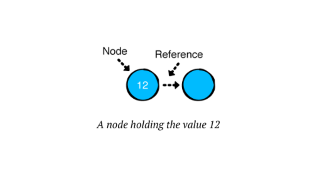
Each node has two components:

• Data: The value we want to store.
• Next: A reference to the next node in the sequence.

Unlike arrays, Linked Lists are dynamic in size, offering efficient insertions and deletions at any position in the list.

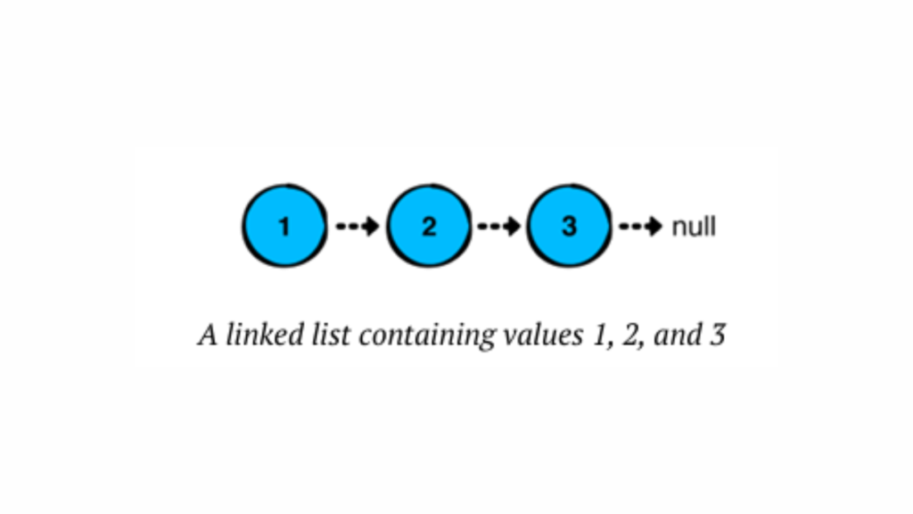
In a linked list, each node stores a value and points to the next node in the chain. The last node in the sequence points to “null,” indicating the end of the list.

Linked lists have several advantages over arrays or ArrayLists in Kotlin:

• Quick insertions and removals at the front of the list.
• Consistent performance for operations, especially for inserting or removing elements anywhere in the list.

Types of Linked Lists

1. Singly Linked List – Each node points to the next node in the sequence (we’ll focus on this one & only for insertion operations).
2. Doubly Linked List – Each node has a reference to both the next and the previous node.
3. Circular Linked List – The last node points back to the first node, forming a loop.

Why Use Linked Lists?

Before we dive into the code, let’s understand why we might choose Linked Lists over arrays:

1. Dynamic Size – No need to specify a fixed size upfront.
2. Efficient Insertions/Deletions – Adding or removing elements doesn’t require shifting other elements.
3. Memory Efficiency – Uses only as much memory as needed.

However, Linked Lists have their trade-offs. Accessing elements is slower compared to arrays because you can’t directly access an element by an index – you have to traverse the list.

Building a Singly Linked List in Kotlin

Now that we understand what Linked Lists are, let’s build one step-by-step in Kotlin! We’ll create the following:

1. Node Class – Represents each element in the list.
2. LinkedList Class – Manages the nodes and provides functionality to add, remove, and display elements.

Defining the Node Class

Each node needs to store data and a reference to the next node. Here’s our Node class:

// We define a node of the linked list as a data class, where it holds a value and a reference to the next node.

data class Node<T>(var value: T, var next: Node<T>? = null) {
    override fun toString(): String {
        return if (next != null) {
            "$value -> ${next.toString()}"
        } else {
            "$value"
        }
    }
}

fun main() {
    val node1 = Node(value = 1)
    val node2 = Node(value = 2)
    val node3 = Node(value = 3)

    node1.next = node2
    node2.next = node3   //here node3 points to null at last, as per our code we only print its value
    println(node1)
}

//OUTPUT

1 -> 2 -> 3

Here, we defined a generic Node class for a linked list in Kotlin. Each Node holds a value of any type (T) and a reference to the next Node, which can be null. The toString() method provides a custom string representation for the node, recursively displaying the value of the node followed by the values of subsequent nodes, separated by ->. If the node is the last in the list, it simply shows its value.

Have you observed how we constructed the list above? We essentially created a chain of nodes by linking their ‘next’ references. However, building lists in this manner becomes impractical as the list grows larger. To address this, we can use a LinkedList, which simplifies managing the nodes and makes the list easier to work with. Let’s explore how we can implement this in Kotlin.

Creating the LinkedList Class

Let’s create our LinkedList class and add core functionalities like adding nodes and displaying the list.

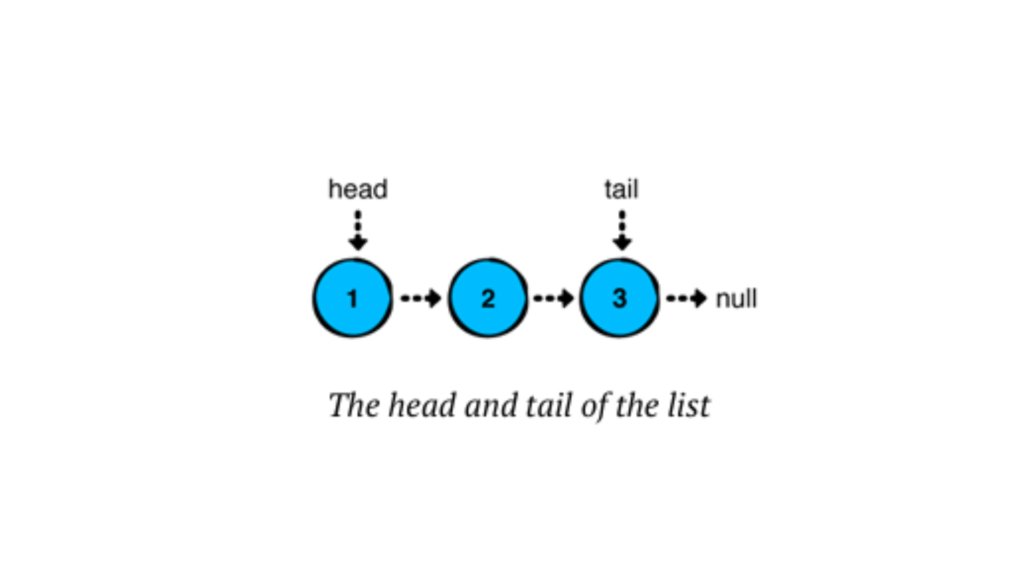
Basically, a linked list has a ‘head’ (the first node) and a ‘tail’ (the last node). In a singly linked list, we usually only deal with the head node, although the tail node can also be relevant, especially when adding elements at the end. The tail node becomes more important in doubly linked lists or circular linked lists, where it supports bidirectional traversal or maintains circular references. However, here, we will use both nodes in a singly linked list.

class LinkedList<T> {
    private var head: Node<T>? = null
    private var tail: Node<T>? = null
    private var size = 0

    fun isEmpty(): Boolean {
        return size == 0
    }
     // to print nodes in linkedlist
    override fun toString(): String {
        if (isEmpty()) {
            return "Empty list"
        } else {
            return head.toString()
        }
    }
}

Here, a linked list has a ‘head’ (the first node) and a ‘tail’ (the last node). We’ll also store the list’s size in a ‘size’ property.

Adding values to the list

Now, let’s develop a way to manage the nodes in our list and focus on adding values. There are three common approaches to inserting values into a linked list, each offering different performance benefits:

• Push: Inserts a value at the start of the list.
• Append: Adds a value to the end of the list.
• Insert: Places a value after a specified node in the list.

We’ll implement these methods step by step and analyze their performance.

Push Operations

Inserting a value at the beginning of the list is called a push operation or head-first insertion. The implementation for this is remarkably straightforward.

To achieve this, add the following method to our LinkedList class:

// This function is used to insert a new element at the first position in the linked list.
// This is a head-first insertion.
fun pushAtHead(value: T) {
    head = Node(value, next = head) // The previous head value (i.e., null if the list is empty) is assigned to the next node.

    // If the list is empty (i.e., tail is null), we add the new node and assign it to the tail.
    // If the tail is not null, we add the new element and assign it to the head (as done above).
    if (tail == null) {
        tail = head
    }

    size++ // Whenever a new node is added, the size is increased by one.
}

What happens here is that when we push into an empty list, the new node becomes both the head and the tail. Since the list now contains one node, we increase the size.

We will run this code, but I have a question for you: Should we always run this code in the main function? I mean, should we always copy and paste it into Android Studio or Kotlin Playground? What if, in the future, we want to revisit or refer to it? The answer is simple—we can use special Kotlin features like infix functions and higher-order functions. By doing this, we can create a Runner class and add different functionalities using infix and higher-order functions. This approach will make the code easier to understand and manage in the future. Without further delay, let’s implement it, and I’ll explain how it works.

First of all, create a new file and name it LinkedListRunner.kt. Then, add the following code:

fun main() {
    // Push operation at the first position in the linked list.
    "push" example {

        val list = LinkedList<String>()

        list.pushAtHead("amol")
        list.pushAtHead("satara")
        list.pushAtHead("bajirao")
        list.pushAtHead("pune")

        println(list)

    }
}

// This infix function is used to print an example description and then execute the provided function.
infix fun String.example(function: () -> Unit) {
    println("----- Example of $this -----")
    function()
    println()
}

Here,

Infix Function (“push” example{..})

An infix function allows you to call a function in a cleaner and more readable way, without parentheses and dots. In this case, "push" example {...} is an example of an infix function.

How it works:

• "push" is a string, and when combined with example, it invokes the example function.
• The infix keyword enables the usage of this function in a special syntax: a infixFun b instead of a.infixFun(b).
• In this function, this refers to the string "push" and is used to print a custom message (like "----- Example of push -----").

Higher-Order Function (String.example())

The example function is also a higher-order function because it takes another function as a parameter.

How it works:

• The example function takes a lambda expression (function: () -> Unit) as a parameter. This is a function that does not take any arguments and returns nothing (Unit is equivalent to void).
• Inside example, the function passed (function()) is executed.
• In your code, the block of code inside {} (which modifies the linked list) is the function being passed to example as a lambda.

So, finally, 

• Infix Function: The example function is used with infix notation, making the code more readable. It prints the description "----- Example of push -----" and then runs the provided code block.
• Higher-Order Function: The example function is a higher-order function because it accepts a lambda function as a parameter and executes it inside its body.

Execution Flow will be…,

• The string "push" calls the infix function example.
• The block of code inside {} (which adds items to the linked list) is passed as a lambda to the example function.
• example prints the message "----- Example of push -----", runs the lambda function to manipulate the linked list, and prints the result.

----- Example of push -----
pune -> bajirao -> satara -> amol

This approach is good, but we can improve it further. By using the fluent interface pattern, you can chain multiple push() calls together. To do this, modify the push() method to return LinkedList<T>. Then, add return this at the end, so it returns the list after adding the new element.

Create a new method in LinkedList.kt. The method should now look like this:

// Push operation using chaining.
// Head-first insertion using chaining.
fun pushingAtHead(value: T): LinkedList<T> {
    head = Node(value, next = head) // The previous head value is assigned to the next node.
    
    // If the list is empty (i.e., tail is null), assign the new node to the tail.
    if (tail == null) {
        tail = head
    }
    
    size++ // Increment the size of the list whenever a new node is added.
    return this // Return the updated list to enable chaining.
}

In the main() function of the LinkedListRunner.kt file, you can either create a new method or update the existing one to use the return value of pushAtHead().

"fluent interface for chain pushing" example
    {
        val list = LinkedList<Int>()
        list.pushingAtHead(2).pushingAtHead(3).pushingAtHead(7).pushingAtHead(1)
        println(list)
    }

//Output 
 
----- Example of fluent interface chain pushing -----
1 -> 7 -> 3 -> 2

That’s better..! Now, you can easily add multiple elements to the beginning of the list.

Wait a moment…! What we see here might seem unclear at first, but is it really necessary? Yes, it is! That’s why I’ve covered it here. As we go further, you’ll get used to it, and things will become much clearer.

Append Operations

Next, we’ll focus on the append operation, which adds a value to the end of the list (also known as tail-end insertion).

In LinkedList.kt, we’ll add the following code right below the push() method:

// Append a new node at the last position of the linked list.
// Tail-end insertion.
fun appendAtTail(value: T) {
    // Example: 1 -> 2 -> 3 -> 4
    if (isEmpty()) {
        pushAtHead(value) // If the list is empty, add the new node at the head.
        return
    }
    
    // If the list is not empty, link the new node to the tail and update the tail.
    tail?.next = Node(value)
    tail = tail?.next // Update the tail to the newly added node.
    
    size++ // Increment the size of the list when a new node is added.
}

This code is quite simple:

1. As before, if the list is empty, we need to set both the head and the tail to the new node. Since appending to an empty list is the same as pushing, we can use the push method to handle this for us.
2. For all other cases, we create a new node after the current tail node. The tail won’t be null here because we’ve already handled the empty list case earlier in the code.
3. Since this is a tail-end insertion, the new node becomes the tail of the list.

Now, go back to LinkedListRunner.kt and add the following code at the bottom of main():

"append" example{
        val list = LinkedList<Int>()

        list.appendAtTail(1)
        list.appendAtTail(2)
        list.appendAtTail(3)
        list.appendAtTail(4)

        println(list)
    }
    
    
    //Output
    ----- Example of append -----
    1 -> 2 -> 3 -> 4

You can apply the technique you used for push() to create a fluent interface for append() as well.

// Append using chaining.
// Tail-end insertion using chaining.
fun appendingAtTail(value: T): LinkedList<T> {
    if (isEmpty()) {
        pushAtHead(value) // If the list is empty, add the new node at the head.
        return this
    }

    // If the list is not empty, link the new node to the tail and update the tail.
    tail?.next = Node(value)
    tail = tail?.next // Update the tail to the newly added node.

    return this // Return the updated list to enable chaining.
}

Whether you find it useful or not, just think about the possibilities of chaining both push and append together. Or, feel free to have some fun experimenting with it.

Insert Operations

The third and final operation for adding values is insert(afterNode: Node<T>). This operation allows us to insert a value at a specific position in the list, and it involves two steps:

1. Locating the node where the value should be inserted.
2. Inserting the new node right after the located node.

First, we’ll write the code to find the node where we want to insert the value.

In LinkedList.kt, add the following code just below the append() method:

// Get the node at the specified index.
fun nodeAt(index: Int): Node<T>? {
    var currentNode = head
    var currentIndex = 0

    // Traverse the list until the node at the specified index is found.
    while (currentNode != null && currentIndex < index) {
        currentNode = currentNode.next
        currentIndex++
    }

    return currentNode // Return the node at the specified index, or null if not found.
}

nodeAt() retrieves a node from the list based on the given index. Since we can only start from the head node, we need to traverse the list step by step. Here’s how it works:

1. We start with a reference to the head node and keep track of the number of steps taken.
2. Using a while loop, we move through the list until we reach the desired index. If the list is empty or the index is out of range, it will return null.

Next, we will insert the new node. To do this, add the following method below nodeAt().

// Insert a new node with the specified value after the given node.
// If the node is the tail, the new node is appended at the tail.
fun insertAt(value: T, afterNode: Node<T>): Node<T>? {
    if (tail == afterNode) {
        appendAtTail(value) // If afterNode is the tail, append the new node at the tail.
        return tail!! // Return the updated tail.
    }

    // Create a new node and link it to the node after the given node.
    val newNode = Node(value = value, next = afterNode.next)
    afterNode.next = newNode // Update the next pointer of the afterNode to the new node.
    
    size++ // Increment the size of the list.
    return newNode // Return the newly inserted node.
}

Here’s what we’ve done:

1. If the method is called with the tail node, we use the append method, which updates the tail.
2. Otherwise, we create a new node and link it to the next node in the list.
3. We update the specified node to point to the new node.

To test this, go to LinkedListRunner.kt and add the following code at the bottom of main().

"linked list insert At perticular index " example {

        val list = LinkedList<Int>()
        list.pushAtHead(1)
        list.pushAtHead(2)
        list.pushAtHead(3)

        println("list before insert $list")

        var middleNode = list.nodeAt(1)!!

        for(i in 1..3){
            middleNode = list.insertAt(-1 * i, middleNode)!!
        }

        println("After inserting $list")
    }
    
    
    //Output
    ----- Example of linked list insert At perticular index  -----
    list before insert 3 -> 2 -> 1
    After inserting 3 -> 2 -> -1 -> -2 -> -3 -> 1

Great job! You’ve made excellent progress. To recap, you’ve implemented the three operations for adding values to a linked list, as well as a method to find a node at a specific index.

Conclusion

We’ve explored the key insertion operations in linked lists, along with the foundational concepts and structure that make them an essential part of data management. Understanding these operations provides a solid base for working with linked lists in various scenarios. As you continue to practice, you’ll gain more proficiency in implementing and manipulating linked lists, further enhancing your problem-solving skills in Kotlin.